LLM Cost Control: A Practical Playbook for Keeping Unit Economics Sane

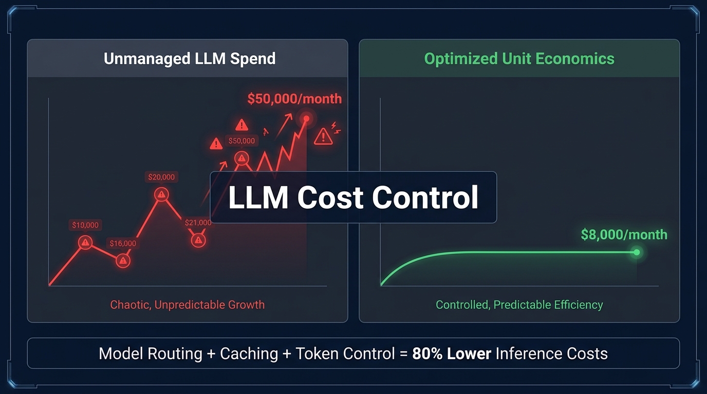
The bill arrives at the end of the month, and nobody budgeted for it. A team ships a new AI feature — customer support automation, a copilot sidebar, an AI-powered search — and within six weeks the inference spend has quietly climbed into five figures. The per-token price looks fine in isolation. GPT-4o runs at $2.50 per million input tokens. Gemini 2.0 Flash is a rounding error at $0.10. But somewhere between the pricing page and the production environment, a gap opens up between what the tokens cost and what the feature actually earns.

This is the defining finance problem for AI-first product teams in 2026: LLM inference is not infrastructure overhead. It is cost of goods sold — a variable, usage-correlated expense that moves in direct proportion to how much customers use the product. That is a fundamentally different economic shape than the server bills traditional SaaS companies have managed for two decades, and most finance and engineering teams are still catching up to the implications.

This post is not about whether AI is worth the cost. It is about the mechanics of keeping the economics sane once you commit to building on top of LLMs at scale. We will cover the structural math that most teams get wrong early, the specific technical levers that actually move the needle — model routing, caching, output token control, fine-tuning — and the FinOps and pricing practices that prevent a successful product from becoming an unprofitable one. Every number cited here is drawn from production-environment benchmarks and current 2026 pricing realities.

Why LLM Costs Are Structurally Different From Classic SaaS COGS

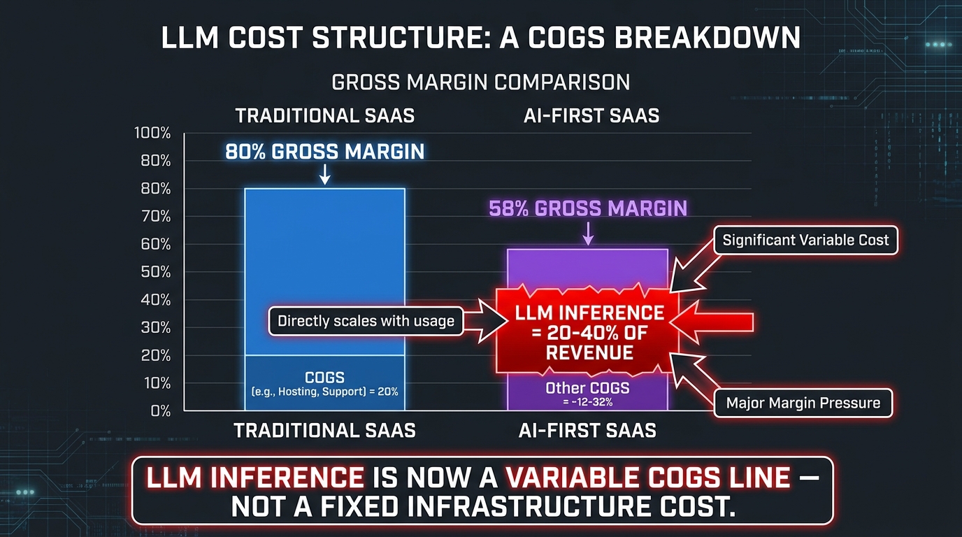
In classic SaaS, the infrastructure cost of serving an additional user is effectively flat beyond the base server provisioning. Storage costs a little more. Compute scales slowly. The marginal cost of one more customer using the product is close to zero, which is why SaaS gross margins of 78–85% are considered normal and defensible.

AI-first SaaS breaks that model. Every user action that triggers an LLM call costs something. Not a fixed something — an unpredictable, usage-dependent something that scales with query complexity, conversation length, output verbosity, and how many agentic steps the workflow takes. The result is structurally lower gross margins: AI-native B2B SaaS companies in 2026 typically report gross margins in the 55–70% range, with the gap from traditional SaaS explained almost entirely by inference COGS.

The COGS reality check

For companies where LLM inference is core to the product — not a peripheral feature — inference costs typically represent 20–40% of revenue. In aggressive growth phases, or when a product leans heavily on frontier models, that figure can push higher. The companies achieving 70%+ gross margins in this space are not doing so because they have negotiated better API prices. They are doing so because they have engineered their inference architecture deliberately, from the model tier all the way to how they price and gate usage.

The key reframe here is treating inference as a production input — something closer to raw materials than to hosting fees. A manufacturer of physical goods manages the cost of steel, fabric, or microchips per unit of output. An AI product company needs to manage the cost of tokens per unit of user value delivered. That framing changes how you instrument your systems, how you evaluate architectural decisions, and how you think about product features.

Why per-token pricing obscures the real problem

The headline API prices — $2.50 per million input tokens, $10 per million output tokens for GPT-4o, or $0.10/$0.40 for Gemini 2.0 Flash — create a false sense of cheapness. The math looks manageable until you multiply through. A customer support application that handles 50,000 conversations per month, averaging 2,000 tokens of input context and 500 tokens of output per exchange, will consume 100 billion input tokens and 25 billion output tokens monthly. At GPT-4o pricing, that is $250,000 in input costs plus $250,000 in output costs — $500,000 per month before a single line of surrounding infrastructure.

Most production teams do not start at that scale, but the point is the directionality: costs compound with usage in a way that fixed infrastructure bills do not. The per-token number looks safe at low volume. It becomes a strategic problem the moment a product succeeds.

The Unit Economics Math: Cost Per Query, Task, and User

Before you can control LLM costs, you need to measure them at the right granularity. Most teams start by looking at the monthly invoice from their API provider. That is the right starting point, but it is the wrong ending point. The actionable metric is not total spend — it is cost per unit of value delivered.

Three layers of cost measurement

There is a hierarchy to LLM cost measurement that mirrors the hierarchy of business decision-making:

• Cost per inference request: The raw unit. Input tokens plus output tokens multiplied by the model’s per-token rate. This is what the API provider charges and what shows up in log files. It is necessary but insufficient because a “request” is not a unit of business value.
• Cost per completed task: How much does it cost, in aggregate LLM spend, to successfully complete one coherent unit of work — answer one customer question, generate one report, complete one code review? This is the metric that maps to user value and allows you to determine whether a feature is economically viable at a given price point.
• Cost per active user per month: The metric that connects to your financial model. If your product charges $30/month per seat and your average user’s LLM usage costs $18/month to serve, you have a contribution margin problem that no amount of growth will fix.

Teams that only track cost per inference miss the aggregation effects of multi-step workflows. Teams that only track total monthly spend cannot identify which features or user segments are the economic culprits. Both layers are necessary.

Building a cost-per-task baseline

The practical starting point is tagging every LLM API call at the application layer with metadata: which feature triggered it, which user segment it belongs to, and which workflow step it represents. This does not require sophisticated tooling at the start — a structured logging schema that captures model name, token counts, and a feature/workflow identifier is enough to begin building the baseline.

Once you have two to four weeks of tagged data, patterns emerge quickly. In most production applications, 10–20% of request types account for 60–80% of total inference spend. These high-cost outliers — typically long-context operations, verbose generation tasks, or heavily agentic workflows — are where optimization effort returns the most. Trying to optimize across the board before identifying these clusters is a common mistake that produces marginal savings at high engineering cost.

The Agentic Multiplier: How Multi-Step AI Workflows Blow Up Your Token Budget

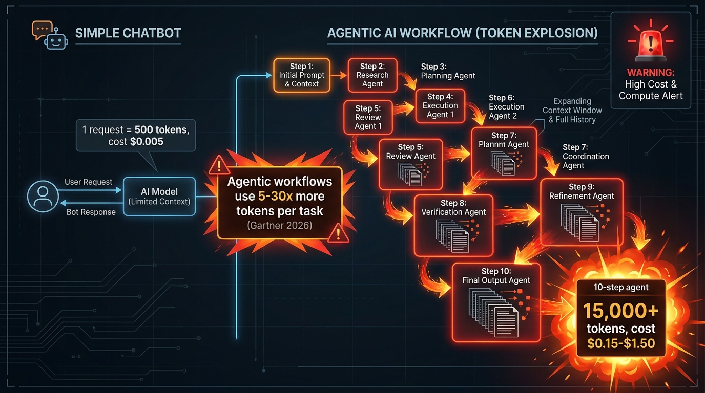
If there is one development that has most disrupted LLM cost planning in the past year, it is the proliferation of agentic workflows. When you build a multi-step agent — a system that plans, uses tools, executes intermediate steps, reflects on results, and iterates — the token economics change dramatically compared to a simple chat interface.

Gartner’s March 2026 analysis found that agentic models require 5–30 times more tokens per task than standard chatbots. The mechanism is structural: most agentic frameworks re-send the full conversation history and tool output log at every inference step. A 10-step coding or research agent does not cost 10x a single query — it costs the sum of 10 queries where each successive query carries a larger and larger context window from all previous steps. Token consumption grows faster than linearly with the number of steps.

The real cost of a “simple” agent

To make this concrete: a single 50-step coding and debugging session on a mid-tier model can cost between $0.60 and $6.00, depending on model selection and context management. Users running multiple such sessions per day can accumulate costs of $400–$1,500 per month per heavy user — even as base per-token prices have declined. In scenarios where agents are poorly bounded and can run unbounded loops, reported monthly bills have reached $4,000+ for individual users before alerting systems caught the issue.

The cost problem with agentic systems is not that inference is expensive per step. It is that the cumulative context growth makes each successive step progressively more expensive, and most teams do not model this trajectory when they approve the architectural decision to build an agent.

Agentic cost controls that actually work

Controlling agentic costs requires intervention at the architecture level, not just at the token pricing level:

• Step-count caps: Hard limits on the number of agent iterations per session. This sounds blunt but is effective. Most legitimate tasks complete within a bounded number of steps; runaway loops are almost always errors, not genuinely productive work.
• Context compression between steps: Instead of passing the full raw conversation history to each step, use a summarization pass that compresses earlier steps into a compact representation. LLMLingua-style compression can reduce context token counts by 40–60% with minimal quality loss on well-structured agent tasks.
• Session-level budget alerts: Set cost thresholds per session (e.g., $0.50) that trigger a user notification or a graceful handoff rather than allowing unbounded continuation. This is table-stakes governance for any agentic product with per-seat pricing.
• Hierarchical agent architectures: Use a cheap, fast model for orchestration and routing between steps, and only invoke the frontier model for the specific sub-tasks that genuinely require its capabilities. An orchestrator running on Gemini 2.0 Flash Lite at $0.075 per million tokens coordinating calls to GPT-4o only when needed can cut per-session costs dramatically.

Model Routing and Cascade Architectures

Model routing is the highest-leverage single change most production teams can make to their LLM cost structure. The premise is simple: not every query requires your most expensive model. A customer support chatbot handling a question about account settings does not need the same model as one handling a complex multi-step dispute resolution. A code completion request for a three-line function does not need the same capabilities as architectural code review.

The difference in price between routing that code completion to GPT-4o mini at roughly $0.15 per million input tokens versus GPT-4o at $2.50 per million input tokens is approximately 17x. If 70% of your traffic consists of tasks where the cheaper model delivers equivalent quality, your blended cost per request drops by roughly 73% — without any visible quality degradation for users.

Routing vs. cascade: two different architectures

There are two distinct patterns for deploying multi-tier models, and they have different strengths:

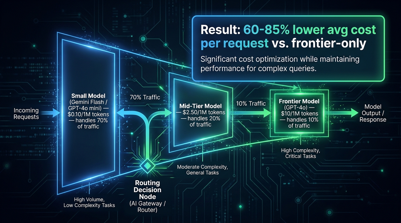
Routing selects a single model before inference runs, based on a classifier that evaluates query complexity, type, or metadata. A routing classifier might direct simple factual questions, format-heavy tasks (like filling a template), and short-context requests to a budget model, while directing open-ended reasoning, long-document tasks, and anything flagged as high-stakes to a frontier model. Done well, routing can handle 60–80% of queries at budget-model cost with no user-visible quality difference.

Cascade architectures run the cheap model first and escalate to a more capable model if the output fails a confidence or quality threshold. The advantage is that you never miss on quality — every query gets the capabilities it needs. The disadvantage is latency: users may notice the two-step delay when escalation triggers. Cascades work well for asynchronous workflows and batch processing but are less suited to real-time interactive features.

Real-world routing savings

Production deployments of model routing consistently report cost reductions in the 45–85% range. One commonly cited configuration routes 90% of traffic to a small model and 10% to a frontier model, reducing average per-request cost by roughly 86% compared to frontier-model-only architecture. The key variable is the quality of the routing classifier: a naive classifier that routes poorly wastes both the cost savings (by sending complex queries to the cheap model) and user trust (by delivering poor results on requests that needed better handling).

Building a good routing classifier requires a labelled dataset of your actual production traffic, typically 500–2,000 examples spanning the quality gradient you care about. The investment pays back quickly at any reasonable query volume. A team processing 5 million queries per month at a 70% routing rate to budget models saves approximately $60,000–$180,000 per month in inference costs at current pricing — enough to justify a dedicated engineering sprint with room to spare.

The model portfolio mindset

The strategic shift here is thinking in terms of a model portfolio rather than a single model contract. Your production architecture should maintain at minimum three tiers: a budget/flash model for simple, high-volume requests; a mid-tier model for moderately complex tasks; and a frontier model reserved for your hardest, highest-stakes operations. The exact models in each tier will shift as the market evolves — the pricing landscape in 2026 looks materially different from 12 months ago — but the three-tier structure is durable.

Semantic Caching and Prompt Caching: The Cost Lever Most Teams Skip

Caching is the most under-deployed cost optimization in production LLM systems, despite having some of the strongest documented savings rates of any technique. There are two distinct forms of caching that matter here, and confusingly, they address completely different parts of the inference pipeline.

Provider-side prompt caching and KV caching

Prompt caching — offered by Anthropic, OpenAI, and Google at the API level — discounts the cost of re-processing token sequences that were seen in recent prior requests. If your application consistently prepends the same system prompt, document, or context block to many requests, the provider only charges full price for processing that prefix the first time; subsequent requests that share the prefix get a discounted rate on those tokens (typically 50–90% cheaper). This requires no changes to your model selection or architecture — only structuring your prompts so that the static prefix comes first and varies last.

The savings here can be substantial for applications with shared context. A document QA application that loads the same 20,000-token knowledge base for every query in a session saves the input cost of those 20,000 tokens on every query after the first. At GPT-4o pricing with caching applied, that is the difference between $0.05 per query and roughly $0.005 — a 10x reduction on the input side for the static portion.

Semantic response caching

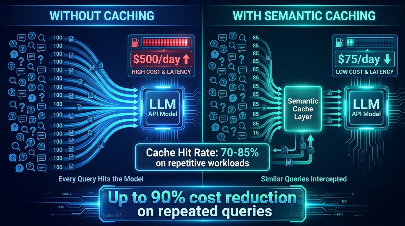
Semantic caching operates at a different layer: it stores the outputs of previous LLM calls and returns cached responses for sufficiently similar new queries, without hitting the model at all. Unlike simple key-value caching (which only matches exact query strings), semantic caching uses embedding-based similarity search to identify when a new query is semantically equivalent to a previous one.

For applications with structurally repetitive traffic — customer support, FAQ systems, internal knowledge base queries, product recommendation engines — semantic cache hit rates of 70–85% are achievable on mature traffic patterns. At an 80% cache hit rate, you are paying for inference on only 20% of requests, which translates to roughly 80% savings on the per-query cost line. In absolute terms, a system handling 1 million queries per day at an average cost of $0.01 per query saves $8,000 per day — $2.9 million per year — from a well-tuned semantic cache.

Implementing caching without sacrificing freshness

The practical challenge with semantic caching is managing staleness. For factual or policy-dependent responses, returning a cached answer that is six weeks old can cause real user harm. The engineering requirement is a cache invalidation strategy: time-to-live policies, version tagging tied to knowledge base or policy updates, and topic-specific TTL differentiation (static product FAQs can cache for weeks; real-time pricing queries should not cache at all).

Tools like Langchain’s caching layer, GPTCache, and infrastructure-level AI gateways from vendors like Portkey, LangFuse, and Helicone all support semantic caching with configurable similarity thresholds and TTL policies. The implementation time for a basic semantic cache on a production system is typically two to five engineering days — a highly asymmetric investment given the potential return.

Output Token Control: The 4x Cost Wedge Most Teams Accept Without Question

Of all the line items in an LLM inference bill, output tokens are the least optimized and the most expensive. Across all major providers, output tokens cost between 3x and 5x more per million than input tokens. GPT-4o charges $2.50 per million input tokens and $10 per million output tokens — a 4x ratio. Claude 3.5 Sonnet runs at similar economics. This is not a coincidence: generating tokens requires sequential computation through the model’s autoregressive architecture, while reading input tokens can be processed in parallel.

Yet in most production systems, output length is treated as a product-determined parameter (“the model should give thorough, helpful responses”) rather than an economic parameter that requires active management. This is a mistake that compounds at scale.

Where output token waste comes from

There are three primary sources of unnecessary output token spend in production systems:

Verbose system prompts that invite verbose outputs. System prompts that say “provide a detailed, comprehensive response” or “explain your reasoning step by step” result in outputs that are 3–5x longer than prompts that say “respond in 2-3 sentences unless the user explicitly asks for more detail.” The difference is a measurable output cost reduction of 40–70% on average query length, without degradation in user satisfaction for the majority of interaction types.

Chain-of-thought reasoning included in the final response. Many applications use chain-of-thought prompting to improve reasoning quality, which is legitimate. The mistake is having the model include the full reasoning trace in the user-visible output. For internal reasoning that feeds into a final answer, using structured prompts that separate the reasoning trace (streamed but not included in the final output) from the final answer reduces output token counts significantly.

No output length constraints in the API call. Every major LLM API supports a max_tokens (or equivalent) parameter that caps output length. Most production applications leave this unconfigured or set it to an arbitrarily high number as a safety margin. Setting this deliberately — by feature type and expected output format — is one of the easiest output cost controls to implement and one of the most consistently ignored.

Output constraints by feature type

The right max_tokens setting varies by use case, and maintaining a per-feature configuration is part of good LLM engineering hygiene:

• Classification and routing tasks: 1–10 tokens. A classification response should return a category label, not an explanation.
• Short-form summarization: 100–300 tokens. Enforce brevity at the API level, not just in the prompt.
• FAQ and customer support answers: 150–400 tokens for most queries, with a mechanism to escalate to longer responses only when explicitly requested.
• Code generation: Size the limit to the expected function or module scope, not to an open-ended maximum.
• Long-form content generation: Where length is genuinely part of the product value, use streaming with in-session limits rather than unbounded generation.

Teams that systematically instrument output lengths and set deliberate per-feature caps consistently report 30–50% reductions in total output token spend without measurable quality degradation in user studies.

Fine-Tuning Small Models for Narrow Tasks

Model routing handles the “which model tier for this query” decision in real time. Fine-tuning addresses a different question: can we take a small, cheap model and train it to perform a specific narrow task at quality that is competitive with a much larger frontier model?

In 2026, the answer is increasingly yes — but with important caveats about what “narrow” means in practice. Fine-tuned small language models in the 1–15B parameter range are delivering near-frontier quality on specific production tasks at 10–100x lower inference costs. The economic case is compelling: once the fine-tuning investment is made (which has dropped dramatically in cost, with many fine-tuning runs achievable for under $100 using cloud training APIs), ongoing inference costs are a fraction of frontier model equivalents.

Where fine-tuning produces clear ROI

Fine-tuning works best when all of the following conditions are met:

• The task is narrow and well-defined. “Answer questions about our product catalog” is fine-tunable. “Be a helpful general assistant” is not — that is what frontier models are for.
• You have high query volume. The ROI calculation for fine-tuning depends on amortizing the training cost across a large number of inference calls. At 100,000 queries per month on a narrow task, even a modest per-query savings of $0.001 returns the training cost in weeks.
• The task has stable, definable quality criteria. If you cannot evaluate whether the fine-tuned model is performing well on the task, you cannot know when it is production-ready or when it has drifted.
• Latency matters. Smaller models are faster. For user-facing real-time features, a fine-tuned 7B model running on dedicated infrastructure can deliver sub-200ms responses that a frontier API cannot match at any price.

Fine-tuning vs. few-shot prompting: a cost comparison

Many teams discover fine-tuning as an alternative to few-shot prompting with large examples embedded in every prompt. If you are currently including 10–20 shot examples in a system prompt to coax good performance from a general model on a specific task, that example overhead adds hundreds of tokens to every single request. Fine-tuning moves those examples into the model weights once, eliminating the per-request overhead entirely. For high-volume narrow tasks, switching from few-shot prompting on a frontier model to fine-tuning on a small model can reduce per-query cost by 95% or more.

The caveat is maintenance: fine-tuned models need to be retrained as the underlying task or data distribution changes. Building a retraining pipeline as part of the initial fine-tuning project — not as an afterthought — is the difference between a fine-tuned model that ages well and one that quietly degrades over time.

LLM FinOps: Attribution, Chargeback, and Governance

Even teams that have implemented excellent technical cost controls frequently discover that governance and attribution are the harder unsolved problems. The question is not just “how do we spend less?” but “who is spending what, on which features, for which users, and is that spend generating proportionate value?”

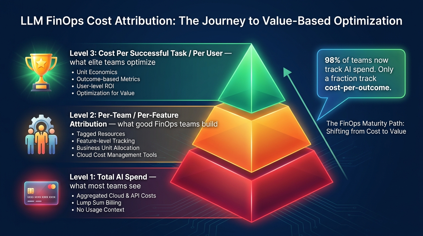
A 2026 industry survey found that approximately 98% of organizations now actively manage and track AI spend in some form. But “tracking” at the aggregate level — watching the monthly invoice number — is very different from the granular attribution that enables real optimization decisions. Only a minority of teams have achieved the level of cost attribution where they can answer: “Feature X on the enterprise tier costs us $0.23 per user per day to serve. Our enterprise tier generates $1.10 per user per day in gross revenue contribution. Is that margin acceptable, and how does it compare across features?”

Building the attribution layer

Effective LLM FinOps starts with tagging every API call at the application layer. The minimum viable attribution schema includes:

• Feature identifier: Which product feature triggered this call (e.g., “support-chat”, “code-review”, “report-generation”)
• Team or cost center: Which engineering or product team owns this feature
• User tier: Free, pro, enterprise — allows unit economics analysis by segment
• Model name and version: Necessary for tracking cost changes across model upgrades
• Token counts: Input and output, captured from the API response

This data flows into a cost allocation system — either a homegrown pipeline or one of the growing number of AI gateway tools (Portkey, Helicone, LangSmith) that provide built-in attribution dashboards. The output is a weekly or daily cost-per-feature report that finance and engineering can both act on.

Showback before chargeback

For organizations running centralized AI infrastructure serving multiple product teams, the question of who pays for what becomes politically charged. The recommended sequencing is showback first, chargeback later.

Showback means making cost attribution visible to each team — “here is what your features cost the organization in inference spend last week” — without actually billing them for it. This phase creates shared understanding, surfaces surprises (“wait, that new RAG feature we shipped costs how much?”), and gives teams time to optimize before financial accountability is applied. Running showback for one to two quarters before moving to chargeback prevents the common failure mode where teams game the system or fight the attribution methodology rather than improving their cost posture.

Per-team budgets and cost anomaly alerts

Once attribution is established, proactive governance requires two additional mechanisms: per-feature or per-team monthly spend budgets, and real-time anomaly alerts when spend diverges from expected patterns. A feature that typically costs $2,000/month in inference and suddenly spikes to $8,000 in a single week has either experienced a traffic anomaly, a prompt regression that is generating longer outputs, or a routing misconfiguration — all of which are worth immediate investigation. Without alerting, these anomalies are discovered only on the monthly invoice, weeks after the issue started.

Pricing Design: Making Revenue Track Inference Costs

Technical cost optimization addresses the numerator in the unit economics equation. Pricing design addresses the denominator. Even perfectly optimized inference costs create margin problems if the pricing model charges a flat fee while costs scale with usage.

The tension is real and well-documented: per-seat, per-month SaaS pricing is what customers understand and what sales teams find easy to sell. But for AI-intensive features, per-seat pricing creates a subsidy problem where heavy users are served at a loss while light users generate outsized margins. Over time, product feedback loops tend to attract more heavy users, worsening the problem.

Usage-based and outcome-based pricing models

AI-first companies are increasingly shifting toward usage-based pricing for their most inference-intensive features, not because it is simpler to sell, but because it is the only pricing structure that naturally aligns revenue with COGS. When a user pays per query, per document processed, or per completed task, every revenue unit corresponds to a cost unit — and the gross margin is structurally protected.

The emerging best practice is a hybrid model: a base subscription fee that covers access and a baseline usage allowance, with metered overage pricing for heavy users. This structure gives customers the cost predictability of subscription pricing while protecting the vendor from the subsidy dynamics of flat-rate unlimited access. It also creates natural product incentives: customers who value the feature enough to use it heavily are also the customers most willing to pay for premium tiers.

Connecting pricing tiers to model tiers

One underused pricing lever is explicitly tiering model quality to pricing tiers. Free-tier users get responses from the cost-optimized model stack; paid tiers get access to better models for complex tasks. This is not a punitive structure — it is a natural alignment of capabilities with willingness to pay, and it has the additional benefit of making the product’s cost structure more transparent to customers.

The prerequisite is that your model routing architecture already exists: if you have built a three-tier model stack, extending it to a customer-visible capability tier requires relatively little additional engineering. The business outcome is a pricing structure where the highest-cost users are also the highest-revenue users, which is how you achieve the margin profile AI-first companies are working toward.

Measuring What Matters: KPIs for LLM Cost Health

The final piece of a functioning LLM cost control system is the right measurement framework. Most teams start with vanity metrics (total tokens consumed, total spend) and arrive at useful metrics (cost per successful task, inference margin by feature) only after a costly period of flying blind. Getting the KPI framework right from the beginning saves months of retroactive instrumentation work.

The core LLM unit economics dashboard

A mature LLM cost health dashboard tracks the following metrics, reviewed at least weekly:

• Cost per successful task (by feature): The primary unit economics metric. Defined as total inference cost for a feature divided by the number of successfully completed tasks (not just requests fired). “Successful” means the user got a usable response — factoring out retries, timeouts, and low-quality outputs that triggered regeneration.
• Inference margin by feature: (Revenue contribution per feature minus Inference COGS per feature) divided by Revenue contribution per feature. This is your gross margin at the feature level, and it is what tells you which features are economically healthy and which need architectural or pricing attention.
• Output token ratio: Average output tokens divided by average input tokens, tracked over time per feature. A rising ratio means responses are getting longer — which may indicate prompt drift, routing changes, or a new user behavior pattern, all worth investigating.
• Cache hit rate: The percentage of requests served from cache. This should be tracked separately for semantic response caches and provider-side prompt caches. A falling hit rate signals traffic pattern changes that may require cache configuration updates.
• Model tier distribution: What percentage of requests are being served by each model tier (budget, mid, frontier). Shifts in this distribution — especially unexpected increases in frontier model utilization — often indicate routing regressions.
• Cost per active user per month (by tier): The metric that connects inference economics to your financial model. If this number is approaching your ARPU for a given pricing tier, you have a structural problem that needs resolution before the next cohort review.

Setting economic thresholds and review cadences

Each of these metrics should have defined acceptable ranges — not just targets to aim for, but thresholds that trigger action when breached. An inference margin below 40% on any feature warrants an immediate review. A cost-per-active-user exceeding 25% of ARPU for any tier triggers a pricing or optimization sprint. Cache hit rates dropping below 50% on a feature that was previously at 75% indicate that something has changed in the traffic pattern.

Weekly reviews of the unit economics dashboard by the combined engineering and product leadership team are not bureaucracy — they are the mechanism by which a successful AI product avoids the margin erosion that has quietly made several high-profile AI feature launches economically unsustainable.

The Optimization Stack: What a Mature LLM Cost Architecture Actually Looks Like

Individual cost controls are valuable in isolation, but the teams achieving 70–80% reductions in effective inference cost are doing so by stacking multiple layers of optimization simultaneously. Understanding how these layers interact — and in what order to implement them — is the difference between incremental savings and structural unit economics improvement.

Layer 1: Measurement and attribution (weeks 1–4)

Nothing else works well until you know what you are optimizing. Implement token-level logging with feature and user tier attribution before doing anything else. This establishes your baseline and identifies the high-spend request types that will benefit most from subsequent optimization layers. Skipping this step and going straight to technical optimization is why many teams report implementing caching or routing without seeing the savings they expected — they optimized the wrong requests.

Layer 2: Prompt and output hygiene (weeks 2–6)

Before routing or caching, clean up the simple inefficiencies: verbose system prompts that inflate output length, missing max_tokens configurations, few-shot examples that could be condensed, and system instructions that invite repetitive or redundant outputs. This layer requires no architectural changes and typically produces 20–40% cost reductions on the requests it touches. It also reduces the baseline that all subsequent optimizations are measured against.

Layer 3: Provider-side caching (weeks 4–8)

Enable prompt caching on your API provider. Restructure system prompts so that static content (knowledge base, policy documents, persona instructions) comes first in the prompt template, maximizing cache prefix overlap across requests. This is a mostly configuration-layer change that delivers 10–40% input token savings on applicable traffic with minimal implementation risk.

Layer 4: Model routing (weeks 6–16)

This is the highest-leverage intervention but also the one requiring the most engineering investment: building and validating a routing classifier on your actual production traffic. The classifier must be evaluated on quality, not just cost — misrouting is worse than over-spending on a frontier model, because it damages user trust. Allocate time for evaluation dataset creation, classifier training, shadow mode testing, and gradual traffic ramp. When done well, model routing delivers 45–85% cost reductions.

Layer 5: Semantic response caching (weeks 10–20)

Semantic caching requires infrastructure (a vector store, an embedding model for query comparison, a cache management layer) and ongoing maintenance (TTL policies, staleness management, similarity threshold tuning). It delivers its best results on traffic with high query repetitiveness — customer support, FAQ, knowledge bases. For applications with highly varied traffic, the implementation cost may not justify the cache hit rate achievable. Evaluate against your baseline traffic distribution before committing.

Layer 6: Fine-tuning and distillation (months 4–9)

Fine-tuning is a longer-horizon investment with strong returns for the right narrow tasks. Identify your top two or three highest-volume, most clearly-defined task types, build an evaluation framework, and invest in a fine-tuning pipeline with retraining capability. The payback period at typical query volumes is weeks to months, but the infrastructure must be in place before the economics make sense at smaller scales.

The stacking effect: A team that implements all six layers on a moderate-volume production application — 2 million queries per month — can realistically move from an average cost of $0.015 per query to $0.003 per query. At that volume, that is a monthly saving of $24,000. At 10 million queries, the same optimization stack saves $120,000 per month — enough to fund a dedicated AI infrastructure team several times over.

Conclusion: The Unit Economics Discipline Is the Product Moat

The companies that will build durable AI businesses over the next three years are not the ones that access the best models — model access is a commodity in 2026. They are the ones that have built the operational and engineering discipline to serve AI features at margins that allow reinvestment, competitive pricing, and survivability through the inevitable cost and revenue fluctuations of a fast-moving market.

The technical levers are well-established now. Model routing can cut costs by 45–85%. Semantic caching can eliminate spend on 70–85% of repetitive traffic. Output token control reduces the most expensive line item by 30–50%. Fine-tuning aligns the cost of narrow, high-volume tasks to the actual computational requirements of those tasks. None of these is novel. What is rare is executing all of them systematically, governed by the right metrics, and aligned with a pricing structure that lets revenue grow with value delivered rather than subsidizing heavy users.

The framing that makes the difference is treating inference not as a server bill but as cost of goods sold. That framing creates the organizational seriousness about LLM unit economics that the problem deserves — measurement systems, weekly reviews, feature-level margin accountability, and pricing design that tracks costs. It also creates the right incentive: every 10% reduction in cost per task is equivalent to a 10% improvement in gross margin, which compounds into competitive pricing power and defensible unit economics at scale.

For most teams, the biggest obstacle is not technical. It is the operational discipline to instrument, measure, and respond to the metrics that tell you whether your AI product is economically viable — not just in the current month, but at 10x the current usage. Building that discipline early, before scale makes the problems harder to fix, is the practical approach to keeping LLM unit economics sane.

Actionable takeaways

• Tag every LLM API call with feature, team, and user tier before implementing any other optimization.
• Audit your system prompts for output length drivers and set explicit max_tokens by feature type.
• Enable provider-side prompt caching and restructure prompts so static content leads.
• Build a three-tier model routing classifier on your actual production traffic distribution.
• Implement semantic response caching for any feature with structurally repetitive query patterns.
• Identify your top two narrow, high-volume tasks as candidates for small-model fine-tuning.
• Add step-count caps and session-level cost budgets to any agentic workflow before it goes to production.
• Review cost-per-task and inference margin by feature weekly, not monthly.
• Evaluate whether your pricing structure aligns per-unit revenue with per-unit inference cost for heavy users.