


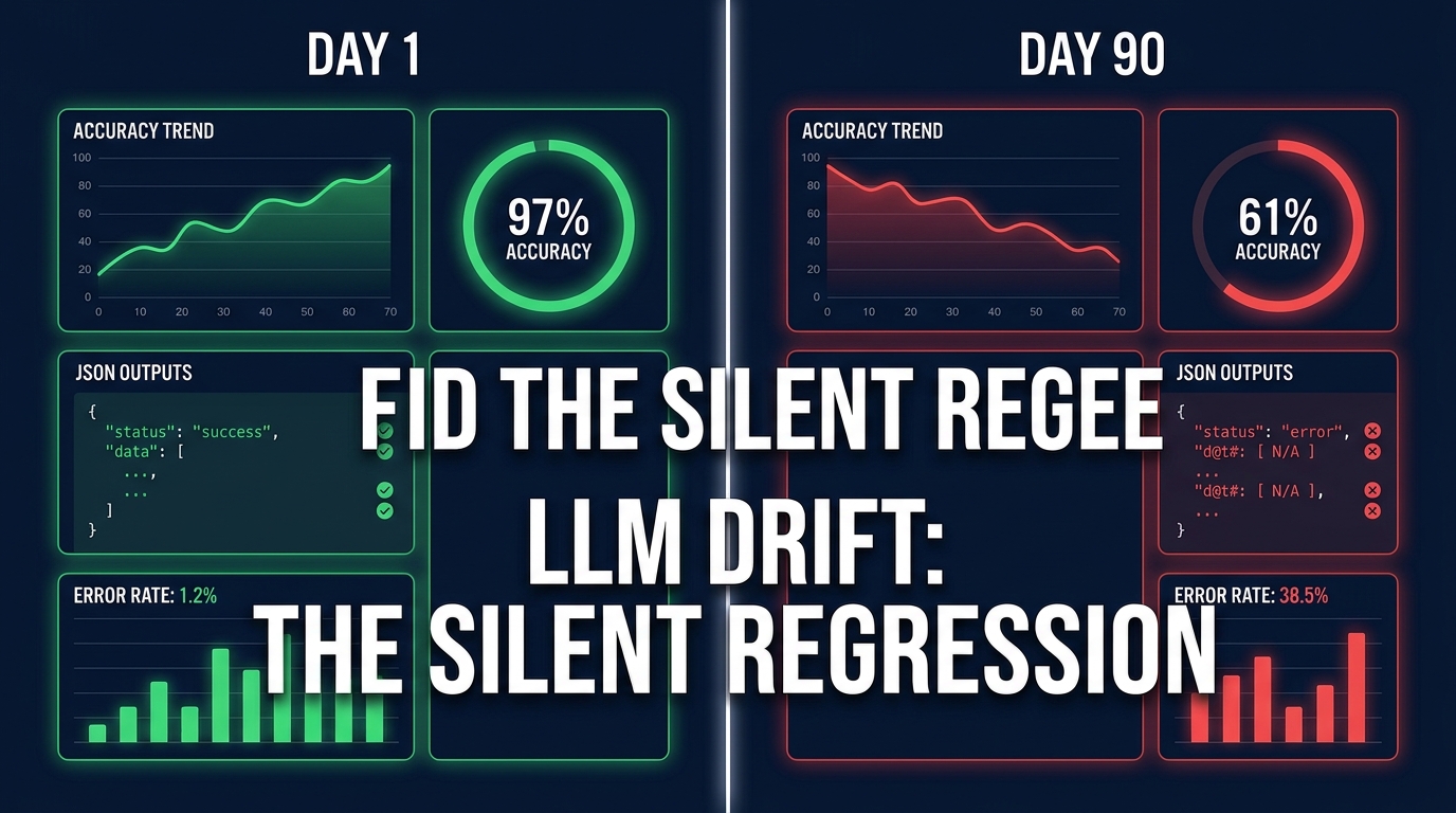

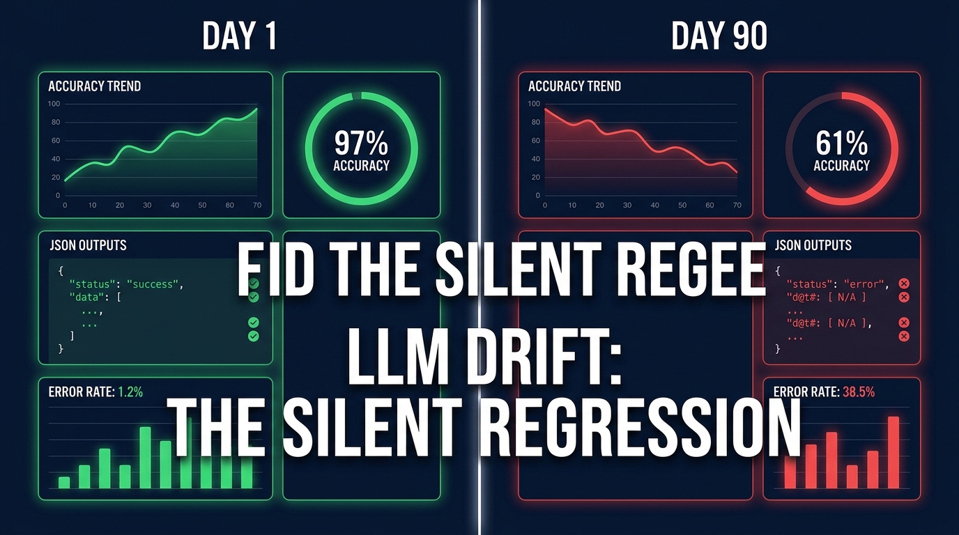
You built the automation. It worked perfectly. You shipped it, measured it, celebrated it — and then, somewhere between week four and week twelve, it quietly started failing.
Not with a crash. Not with an error log. Just a slow, invisible erosion of quality that nobody noticed until a customer complained, a compliance flag appeared, or someone actually read the outputs and realized they’d been subtly wrong for months.
That’s LLM drift. And in 2026, it’s no longer a theoretical concern or an edge case that only affects poorly-built systems. It’s a measurable operational risk affecting the majority of production AI deployments. A 2026 industry survey found that 32.9% of organizations running AI agents in production cite output quality degradation as their top blocker — and the majority of that degradation isn’t caused by bad models. It’s caused by drift that nobody was watching for.
The challenge is that drift doesn’t announce itself. There’s no 500 error, no broken build, no alert in your dashboard. The system keeps running. Responses keep generating. Costs keep accumulating. The only signal is a gradual divergence between what your automation was supposed to do and what it’s actually doing — and by the time that signal is strong enough to catch manually, the damage is done.
This post is about understanding exactly where LLM drift originates, how to build the observability infrastructure to catch it early, and the operational controls that keep your automations stable across the full lifecycle of a production deployment. Not theory — the actual patterns that engineering teams are using right now.
What LLM Drift Actually Is (And What It Isn’t)
Before solving drift, it helps to be precise about what it means. The term gets used loosely to describe any situation where an LLM-powered system behaves differently over time — but not all behavioral change is drift, and conflating them leads to the wrong fixes.
Drift vs. Bugs vs. Intentional Change
A bug is a discrete failure caused by a specific code or configuration error. It has a root cause you can point to, a line number or a commit hash. It’s reproducible and usually binary — either the system works or it doesn’t.
An intentional change is a deliberate update to the model, prompt, or system that was planned, tested, and deployed on purpose. If outputs change because you upgraded your model version last Tuesday, that’s not drift — that’s a release.
LLM drift is neither of those. It’s the gradual, unplanned divergence of system behavior from the established baseline — often without any corresponding code change. The same prompt, the same pipeline, the same infrastructure — but different outputs, declining quality, or degraded task performance over time.
What Changes During Drift
Drift can manifest across multiple dimensions simultaneously, which is what makes it hard to catch. Output quality is the most obvious — accuracy drops, responses become less relevant, structured outputs start violating their schemas. But drift also shows up as changes in tone and style (the model becomes more verbose, or more hedged, or starts refusing requests it previously handled), changes in cost and latency (token counts creep up, response times lengthen), and changes in failure modes (refusal rates spike, hallucination rates increase).
The critical insight is that most drift-related failures look like performance problems, not technical failures. The system is still “working” in the sense that it’s generating responses. They’re just not the right responses anymore.
Why It’s Getting Harder to Ignore
A 2026 study on multi-turn LLM workflows found a 39% average accuracy drop across tested models in multi-turn conversations. GPT-4.1 fell from 91.7% accuracy in single-turn interactions to 70.7% across multi-turn sessions. The same study reported up to 15 percentage points of run-to-run accuracy variation even in ostensibly deterministic settings. When you’re running thousands of automations a day, that variance compounds fast.
The practical implication: if you built your automation six months ago and haven’t actively monitored it since, there’s a meaningful probability it’s performing materially worse today than when you shipped it.
The Four Drift Vectors: Where Instability Actually Originates
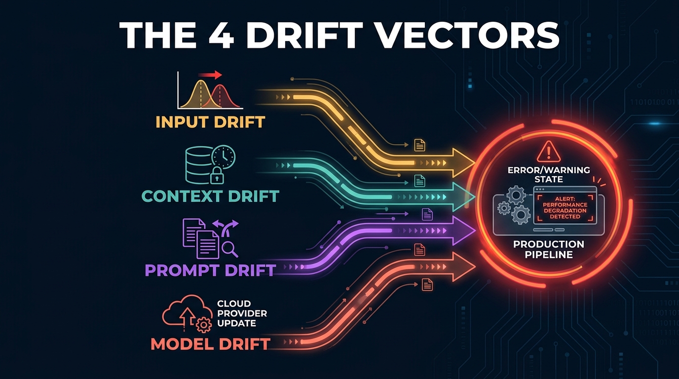
Understanding drift as a single phenomenon is a trap. In practice, drift has four distinct origin points, and each requires a different detection and mitigation approach. Many teams waste time looking in the wrong place because they treat all drift as model drift — when the actual culprit is often something entirely within their control.
Vector 1: Input Drift
Input drift happens when the data flowing into your automation changes character over time. Your users start phrasing requests differently. A new product category gets added to your catalog. A regulatory change shifts the language customers use when contacting support. The underlying LLM hasn’t changed, the prompt hasn’t changed — but the distribution of inputs no longer matches what the prompt was designed to handle.
This is particularly insidious because input drift is often a sign of success. Growing user bases bring more diverse inputs. Expanding product lines introduce terminology the system wasn’t trained to handle. The automation “works” for the original use cases but starts degrading on the new ones — and because the degradation is concentrated in the new inputs, it can take a long time to show up in aggregate metrics.
Detecting input drift requires monitoring prompt embeddings or input feature distributions over time. Statistical tests like the Kolmogorov-Smirnov test, Population Stability Index (PSI), and Jensen-Shannon divergence can identify when incoming inputs have shifted significantly from the baseline distribution used during initial development and validation.
Vector 2: Context Drift
Context drift is the retrieval-layer equivalent of input drift, and it’s arguably more dangerous because it’s completely invisible at the prompt level. This is where most RAG (retrieval-augmented generation) systems quietly fail.
Your vector index was built at a point in time. It contains the documents, policies, product specs, and knowledge articles that existed then, embedded with the embedding model that existed then. But the world doesn’t stay still. Documents get updated. Policies change. Products get discontinued. Old articles that should have been deprecated are still in the index, ready to be retrieved and fed as context to your model.
A 2026 analysis found that 73% of organizations report accuracy degradation in RAG systems within 90 days of initial deployment — driven primarily by retrieval debt: the growing gap between what’s in the index and what’s actually true. The model’s responses remain fluent and confident. They’re just grounded in outdated evidence.
Vector 3: Prompt Drift
Prompt drift is the one that teams cause themselves, usually without realizing it. Someone edits the system prompt to fix a specific edge case. Another engineer tweaks the few-shot examples to improve performance on a subset of inputs. A product manager updates the brand voice instructions. Each individual change seems small and harmless.
But prompts are not modular. Every element of a prompt interacts with every other element, and changes that improve performance on the specific problem that triggered the edit can silently degrade performance on other task dimensions. Prompt drift is effectively accumulated technical debt in your instruction set — and unlike code debt, it doesn’t generate compiler warnings.
The industry is converging on a critical reframe: every prompt change is a release. It needs to be tracked, versioned, and tested against a fixed evaluation set before it ships to production.
Vector 4: Model Drift
Model drift is what most people think of when they hear “LLM drift,” but it’s often the least controllable and, with the right pinning strategy, the most preventable. It happens when the underlying model changes — either through an explicit upgrade or, more commonly, through silent provider-side updates to weights, inference behavior, safety filters, or system-level configurations.
Major providers regularly update their models, adjust their safety layers, and modify inference parameters — sometimes without prominent notification. If you’re using floating aliases like gpt-4 or claude-latest rather than pinned snapshot identifiers, you’re opting into every one of those changes the moment they go live, with no testing and no rollback path.
Model drift can shift tone, change refusal behavior, alter structured output formatting, or introduce new behavioral patterns that break downstream parsing logic. And because the change happens at the provider level, there’s no diff to review — just a before-and-after quality gap that your monitoring either catches or doesn’t.
The Temperature Zero Trap: Why “Deterministic” Settings Give False Confidence
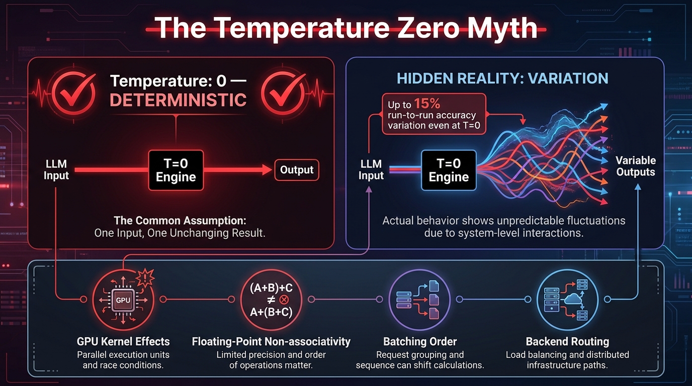
One of the most common stability strategies teams reach for is setting temperature to zero. The logic is straightforward: temperature controls randomness in sampling, so removing randomness should produce identical outputs for identical inputs. If the model is deterministic, drift becomes impossible — or so the reasoning goes.
This is a trap. And it’s important to understand exactly why, because teams that believe in temperature-zero determinism tend to skip the observability work that actually protects them.
What Temperature Actually Controls
Temperature is a parameter that shapes the probability distribution from which the model samples its next token. At temperature 0, you’re selecting the maximum-probability token at each step — which sounds deterministic, but the probability itself is computed by a neural network running on GPU hardware. And that hardware is where the nondeterminism lives.
A March 2026 preprint formalized what practitioners had been observing for years: temperature 0 does not eliminate nondeterminism from LLM outputs. The remaining variation comes from GPU floating-point non-associativity (the order in which floating-point operations are performed affects the result), batch-size effects (different batch sizes can change computation paths), kernel non-invariance, and backend routing to different hardware instances.
The practical effect: a 2026 multi-model study found substantial variability in LLM-as-a-judge scoring even at temperature 0, with completeness scoring showing the largest fluctuations. Different model families responded differently — lower temperatures improved stability for GPT-4o and Gemini, but effects were inconsistent or even counterproductive for some Anthropic models.
The Compounding Effect in Pipelines
The risks compound dramatically in multi-step automations. If each step in a five-step pipeline has even a 5% output variation rate, the probability that the final output of the pipeline exactly matches the baseline is roughly 77%. Run that pipeline hundreds of times a day across an enterprise deployment and you have constant drift introduction — even if every individual component appears stable in isolation.
This is why multi-turn workflows show such dramatic accuracy degradation. A 2026 study measuring performance across extended conversation sessions found that accuracy consistently declined as sessions lengthened — not because the model “forgot” things, but because small variations in earlier outputs propagated forward, compounding through each subsequent step.
What to Do Instead
Temperature 0 is still worth using — it reduces variation even if it doesn’t eliminate it. But it should be treated as one layer in a defense stack, not the whole defense. The teams that actually achieve stable automations combine temperature minimization with output validation, eval-based regression testing, and active monitoring — not instead of those things, but alongside them.
The key mental shift: stop thinking about LLM outputs as files and start thinking about them as measurements. No measurement is perfectly repeatable. The goal is to understand the variance, characterize it, and build systems that are robust to it — not to pretend it doesn’t exist.
RAG Systems and Retrieval Debt: When Your Knowledge Base Lies
RAG systems represent one of the most successful and widely-deployed patterns in enterprise AI — and one of the most fertile grounds for invisible drift. The retrieval layer sits between the user’s query and the model’s response, shaping everything the model knows about the current state of the world. When that layer drifts out of sync with reality, the model’s outputs become confidently, fluently wrong.
The Anatomy of Retrieval Debt
Retrieval debt accumulates in four ways. First, document updates without re-indexing: a policy document gets updated, but the vector index still contains the old chunks. The model retrieves the outdated version and gives outdated advice. Second, deleted content that persists in the index: a product gets discontinued, but its product spec is still retrievable. Customers ask about it, the system answers confidently, the information is wrong.
Third, embedding model drift: the model used to generate your embeddings at index-build time may differ from the model used to embed queries at retrieval time — either because you’ve upgraded the embedding model for queries but haven’t re-embedded the index, or because the embedding model provider has silently updated their weights. This creates semantic misalignment between index and query representations, degrading retrieval relevance.
Fourth, corpus coverage gaps: new information is added to source systems but the re-indexing pipeline is batched or delayed. There’s a window where the knowledge base represents reality imperfectly — and in fast-moving domains like product catalogs, regulatory guidance, or customer support runbooks, that window can be perpetually open.
How Retrieval Drift Manifests in Practice
Support copilots that surface retired runbooks after documentation migrations. Regulatory compliance assistants that cite superseded rule versions. Product recommendation engines that surface discontinued SKUs. These failures share a common structure: the response is fluent, well-structured, and confident. Only someone who knows the underlying ground truth can identify the error. Automated accuracy metrics often miss it entirely because they’re evaluating response coherence, not factual currency.
The operational consequence is severe in regulated environments. A financial services firm whose compliance chatbot cites an old regulatory threshold, or a healthcare organization whose clinical decision-support system references a deprecated treatment protocol — these aren’t quality-of-life issues. They’re liability events.
Managing Retrieval Debt Operationally
The solution isn’t a one-time index rebuild. It’s treating the vector index as a versioned, monitored production artifact with its own SLAs. This means establishing freshness thresholds for document chunks (if a chunk hasn’t been validated against its source document in more than X days, flag it), tracking retrieval overlap metrics over time (if the top-k results for benchmark queries are drifting, your index is changing), and implementing event-driven re-indexing triggers rather than relying solely on scheduled batch rebuilds.
Retrieval quality should also be measured continuously against a fixed benchmark set of queries with known expected retrievals. Changes in Precision@5 or context recall scores on that benchmark set are early warning signals of retrieval drift — detectable before the downstream generation quality degrades enough to be obvious.
How to Build a Drift Detection Stack (The Multi-Signal Approach)
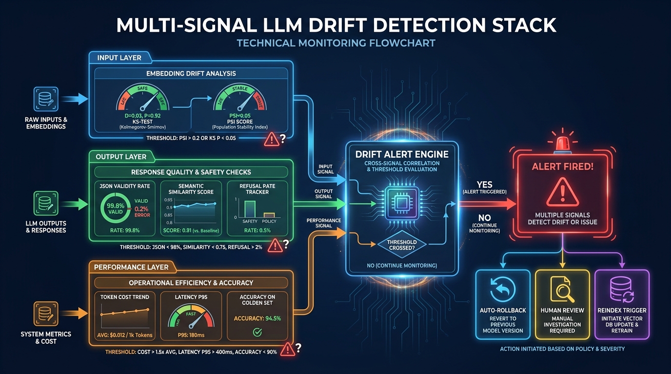
The most common mistake in LLM monitoring is watching a single metric and calling it done. Teams pick accuracy, or latency, or cost — and then wonder why they still get blindsided by drift. Effective drift detection requires multiple signal layers operating simultaneously, because different drift vectors produce different failure signatures.
The Input Layer: Catching Distribution Shift Before It Hits the Model
The first layer monitors the inputs flowing into your system. The goal is to detect when the population of prompts and queries your system is receiving has shifted significantly from the baseline distribution used during development and initial validation.
The practical implementation typically involves embedding incoming prompts into a vector space and comparing the distribution of those embeddings against a stored baseline using statistical distance measures. Kullback-Leibler (KL) divergence, Jensen-Shannon divergence, Wasserstein distance, and Population Stability Index (PSI) are all used in production — PSI is particularly common because it provides an interpretable score and has established industry thresholds (PSI below 0.1 = stable, 0.1-0.2 = moderate shift, above 0.2 = significant shift warranting investigation).
Beyond embedding distance, structural signals like average prompt length, vocabulary novelty (new terms appearing in inputs that weren’t present in the baseline), and query intent classification shifts are all detectable at the input layer without needing to process the output at all. Catching drift here is the cheapest possible intervention — you can respond before bad outputs are generated at scale.
The Output Layer: Measuring What Actually Comes Out
The second layer monitors output quality directly. This is where most teams start, but the challenge is defining “quality” in a way that’s automatically measurable. Several signals are reliably measurable without human review:
JSON and schema validity rates are among the most straightforward. If your automation produces structured outputs, the percentage of responses that parse correctly against the expected schema is a direct quality signal. A validity rate that was 98.5% last month and is now 94% is a concrete, unambiguous drift signal — no LLM-as-a-judge needed.
Semantic similarity to a reference set can be measured by embedding model outputs and comparing them against embeddings of known-good reference outputs. A declining cosine similarity trend indicates the response character is shifting away from the expected baseline.
Refusal rate and abstention rate track what proportion of inputs the model declines to handle or defers on. A spike in refusals can indicate a model safety-layer update, a prompt change that’s triggering guardrails, or input distribution shift that’s pushing queries into territory the model isn’t configured to handle.
Output length distribution is a surprisingly sensitive signal. Models that have drifted — whether through provider updates or context changes — often produce noticeably different output lengths for equivalent inputs. A sudden shift in average token count on stable input types is worth investigating.
The Performance Layer: Cost and Latency as Drift Signals
The third layer monitors system-level performance metrics. These are often already tracked for cost management or SLA compliance, but they double as drift detectors. Token count growth for stable task types suggests the model is generating more verbose responses — possibly due to a model update, a prompt change, or context window inflation. Latency spikes at stable traffic volumes can indicate changes in model inference behavior or routing to different backend capacity. Cost increases without corresponding workload increases are almost always a sign something has changed.
The key is establishing a stable baseline for each of these metrics during a period when the system is known to be working well, then running statistical change-detection algorithms (CUSUM is commonly used) to detect when metrics trend significantly above or below baseline rather than relying on static threshold alerts.
Tying It Together: The LLM-as-Judge Layer
Above the three quantitative layers, a growing number of teams add an automated qualitative evaluation layer using a separate, stable LLM instance to judge output quality on a per-rubric basis. The evaluator LLM scores outputs against specific criteria — factual accuracy, instruction following, tone, citation quality — and these scores are logged as continuous metrics alongside the quantitative signals.
LLM-as-judge evaluation is more expensive than embedding-distance checks, so most teams apply it selectively: on a random sample of production traffic (typically 1-5%), on the fixed golden evaluation set, and on any inputs that triggered anomalies in the quantitative layers. The combination of cheap continuous signal and expensive but high-fidelity qualitative evaluation gives you both the sensitivity to catch drift early and the diagnostic depth to understand what changed.
Eval-Gated CI/CD: Treating Prompt Changes Like Code Changes
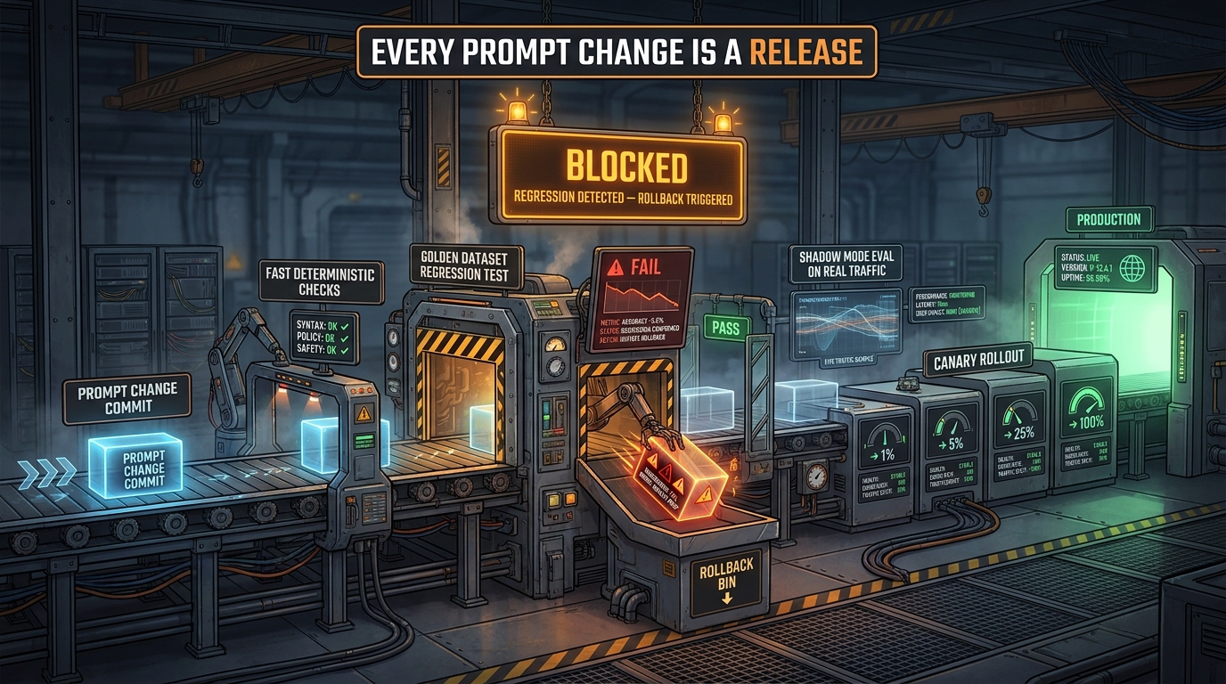
Most software teams have well-established CI/CD practices. Code changes go through linting, unit tests, integration tests, staged deployments, and automated rollback. The systems that enforce this rigor are good at catching software bugs. They’re not designed to catch LLM behavioral regressions — and they miss them, consistently.
Eval-gated CI/CD extends the principle of automated quality gates to the full LLM configuration stack: model version, prompt, retrieval configuration, tool schemas, and inference parameters. The core principle is simple and worth stating plainly: no LLM configuration change ships to production without passing an automated evaluation gate.
Building the Golden Dataset
The foundation of an eval-gated pipeline is a versioned golden dataset — a curated set of input/expected-output pairs (or rubric-scored inputs) that represent the full range of tasks the automation is responsible for. This dataset needs to be stable enough to serve as a reliable regression baseline, comprehensive enough to catch regressions across all major task dimensions, and diverse enough to include known edge cases and challenging inputs.
Building this dataset is unglamorous work, but it’s the single highest-leverage investment in LLM operational stability. Teams that skip it are flying blind — they have no principled way to know whether a prompt change improved, degraded, or had no effect on system quality across the full task distribution. Teams that maintain a good golden dataset can evaluate any change against a stable, repeatable standard.
The dataset itself should be versioned and source-controlled. It changes — new edge cases get added, outdated examples get retired — but those changes should be deliberate and tracked. An unlabeled, unversioned eval set is nearly as dangerous as no eval set at all.
The Gate Structure
The most effective eval-gated pipelines run in multiple stages, ordered from cheapest to most expensive so that fast failures happen early:
Stage 1 — Fast deterministic checks: Schema validation on expected output formats, length bounds checks, format compliance tests. These run in seconds and catch structural regressions immediately.
Stage 2 — Golden dataset regression: Full evaluation against the versioned golden dataset using the primary quality metrics. A change that drops the primary task accuracy score below a configured threshold automatically blocks the merge or deployment. The threshold should be set based on empirical understanding of what score differences are meaningfully significant versus within normal variance.
Stage 3 — Cost and latency projection: Based on sampled outputs from the golden dataset evaluation, project the expected cost and latency impact at production scale. Changes that would meaningfully increase token spend or degrade latency SLAs get flagged for review.
Stage 4 — Safety and policy review: For organizations in regulated industries or with explicit content policies, a separate safety evaluation run assesses whether the change introduces new categories of problematic output. This often involves running a separate battery of red-team test cases alongside the standard golden set.
What Triggers the Gate
A common mistake is running evaluations on every commit, regardless of whether the commit actually touches anything that affects LLM behavior. This creates evaluation fatigue, burns token budget unnecessarily, and slows down development. The better pattern is selective triggering: eval gates only fire when a change touches a prompt file, a model configuration, a retrieval configuration, a tool schema, or other components that directly affect generation behavior. Pure infrastructure or monitoring changes don’t need LLM evaluation.
For changes that are clearly risky — model version upgrades, major prompt restructuring, retrieval index changes — many teams run extended evaluation sweeps on nightly or weekly cadences using a larger, more expensive eval suite that couldn’t run on every PR but is thorough enough to catch subtle regressions.
Model Version Pinning and Prompt Versioning as Operational Discipline
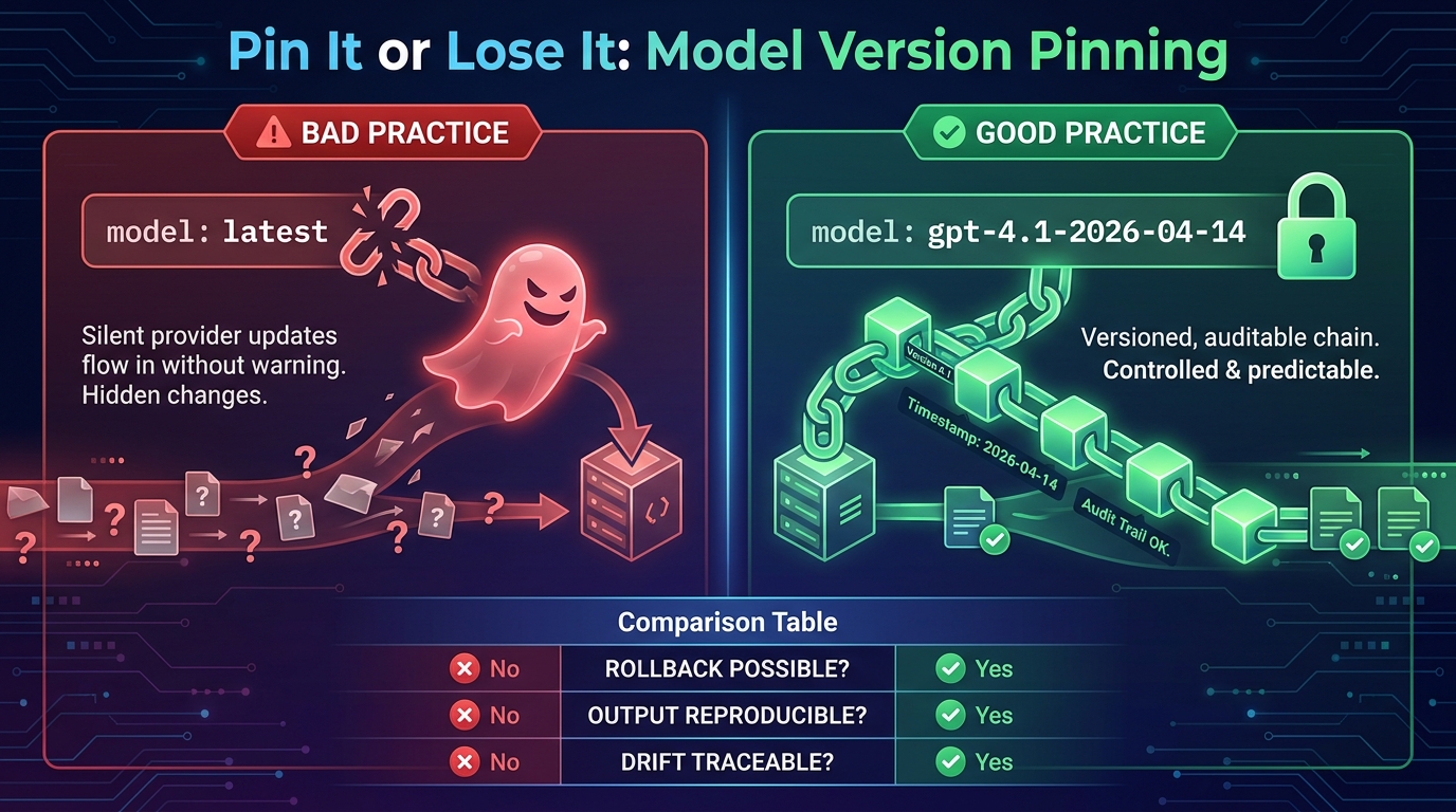
If eval-gated CI/CD is the process that prevents regressions from shipping, version pinning is the infrastructure that makes regression detection possible in the first place. Without it, you can’t reproduce a past behavior, you can’t isolate the cause of a regression, and you can’t roll back safely.
Model Version Pinning
The rule is simple and non-negotiable for production systems: use explicit, dated model identifiers in production, never floating aliases.
Floating aliases like gpt-4, claude-3-opus, or latest are convenience labels maintained by the provider that point to whichever version of the model the provider currently considers canonical. When the provider updates the underlying model — and they do, regularly — your floating alias automatically follows the update. Your production configuration didn’t change. Your model did.
Explicit snapshot identifiers like gpt-4.1-2026-04-14 are immutable. They point to a specific model checkpoint that won’t change without your explicit action. This gives you three things that floating aliases can’t: the ability to reproduce any past behavior for debugging or auditing, a clear demarcation between “the system before the model change” and “the system after,” and a rollback path if a model update introduces regressions.
Maintaining pinned versions requires periodic active upgrade decisions — you need to test new model versions, evaluate them against your golden dataset, and explicitly choose to upgrade. That’s more work than letting aliases float. It’s also exactly the kind of operational discipline that keeps automations stable. Treat every model upgrade like a software release: test it, stage it, roll it out gradually, and keep the rollback path warm.
Prompt Versioning
Prompts should be treated as production artifacts, not strings embedded in application code. The practical implementation looks like this:
Prompts live in a dedicated prompt registry — a source-controlled store where each prompt has an identifier, a version history, and metadata including the model version it was last validated against, the eval scores at time of validation, and the owner responsible for it.
Each production deployment references specific prompt version identifiers, not just the latest content. When a prompt needs to change, the change goes through the same eval-gated pipeline as a model version change: write the new version, run the golden dataset evaluation, compare against the current production version’s baseline scores, and promote only if it passes.
Every production request logs the prompt version and model version used to generate the response. This means any production output is fully reproducible and attributable — a prerequisite for compliance in regulated industries and a fundamental requirement for meaningful post-incident investigation in any context.
The Full Execution Context
Pinning and versioning should extend beyond just model and prompt. The full execution context — model version, prompt version, embedding model version, retrieval index build timestamp, tool schema version, temperature and other inference parameters — should be captured as a snapshot for every production run. This is what makes it possible to say with confidence “here is exactly what ran to produce this output” — a statement that’s increasingly required for enterprise governance and increasingly difficult to make without disciplined versioning infrastructure.
Canary Deployments and Shadow Mode for LLM Changes
Even with rigorous offline evaluation, production behavior can surprise you. Real users generate inputs that don’t appear in your golden dataset. Edge cases that seemed rare in testing turn out to be common in production. Latency that was acceptable in isolation becomes problematic under load. This is why the industry has converged on a staged rollout pattern for LLM changes that mirrors the canary deployment practices established in software engineering, with important adaptations for the characteristics of LLM systems.
Shadow Mode: The Zero-Risk First Stage
Shadow mode is the safest way to evaluate a changed LLM configuration against real production traffic before any users see its outputs. In shadow mode, incoming production requests are duplicated: the current production configuration handles the request and returns its output to the user, while the candidate configuration simultaneously processes the same request and generates an output that nobody sees.
The two outputs are logged, compared, and evaluated offline. Shadow mode reveals regressions that offline eval missed — not because the offline eval was wrong, but because production inputs are always more varied and surprising than curated test sets. Shadow evaluation runs for long enough to accumulate a statistically meaningful sample across the full input distribution, including the tail cases that appear infrequently but matter most.
Shadow mode costs money — you’re running double the inference — but it’s cheap insurance. Running shadow evaluation for 48-72 hours on a new model version before any live exposure catches the vast majority of production regressions before they affect users. The cost of the shadow eval is almost always lower than the cost of a production rollback or the reputational impact of visible quality degradation.
Canary Rollouts: Staged Live Exposure
After shadow evaluation passes quality thresholds, the candidate configuration moves into canary rollout. The standard pattern in 2026 for LLM configuration changes is a staged traffic ramp: 1% → 5% → 25% → 100%, with mandatory hold periods at each stage for quality metrics to stabilize before proceeding.
The hold periods matter. Quality metrics for LLM systems don’t always degrade immediately — some regressions only manifest when the system encounters specific input patterns that appear at a certain traffic volume. A 1% canary might not surface a problem that becomes apparent at 5%. Each stage needs to run long enough to collect a representative sample, typically 24-48 hours per stage for most production automations.
For high-stakes workloads — compliance-critical automations, customer-facing financial tools, clinical decision support — the initial canary percentage should be much smaller, sometimes as low as 0.1%, and the hold periods much longer. The cost of getting it wrong at scale justifies the slower rollout.
Automated Rollback Thresholds
Automated rollback should be configured before any canary starts — not decided retroactively when something goes wrong. Rollback thresholds should be established for the metrics that matter most: output quality scores, refusal rates, schema validity rates, latency P95, and cost per task. If any of these metrics cross the configured threshold during a canary rollout, the system automatically reverts traffic to the previous configuration.
The previous configuration should be kept warm — actively running and ready to receive full traffic — for the entire duration of the canary and for a defined period after full rollout. Rollback should be a traffic routing change that takes seconds, not a code deploy that takes minutes. In practice, this means the “rollback path” needs to be built into the deployment architecture as a first-class feature, not an afterthought.
When to Escalate: Thresholds, Alerts, and Human-in-the-Loop Gates
Not all drift is created equal, and not all drift requires the same response. One of the practical challenges in building drift detection infrastructure is avoiding alert fatigue — a system that fires too many alerts of unclear priority trains teams to ignore it. Effective drift management requires a tiered response model: automated handling for well-characterized drift patterns, human escalation for ambiguous or high-stakes situations, and immediate circuit-breaking for severe regressions.
Tiering the Response
Tier 1 — Monitor and log: Minor drift signals that fall within acceptable variance ranges. Output length trending slightly higher than baseline. Embedding distance scores showing early movement. JSON validity at 97% against a baseline of 99%. These signals go into the monitoring dashboard and feed into trend analysis, but don’t trigger active alerts. Teams review them in weekly operations reviews.
Tier 2 — Alert and investigate: Meaningful but not critical drift. Accuracy on the golden evaluation set drops by more than 5 percentage points. Refusal rates increase by more than 2x baseline. Retrieval overlap scores on benchmark queries decline by more than 15%. These trigger automated alerts to the team responsible for the automation and initiate a structured investigation: identify the drift source, characterize the impact, and determine the appropriate remediation path.
Tier 3 — Circuit break and escalate: Severe regressions requiring immediate action. Schema validity drops below 90%, meaning a significant fraction of outputs are malformed. Accuracy falls below the minimum acceptable threshold for the use case. Cost or latency spikes to multiples of baseline, suggesting a runaway condition. At this tier, automated circuit-breakers should pause or reroute traffic, and the on-call escalation path activates immediately.
Human-in-the-Loop Gates for High-Stakes Contexts
For automations operating in regulated, safety-critical, or high-value contexts, some decisions should not be fully automated even when drift signals are clear. Before promoting a new model version in a clinical decision-support context, before changing a compliance assistant’s prompt in a financial services context, before updating the retrieval index for a legal research tool — these changes benefit from explicit human sign-off in addition to automated eval gates.
The human-in-the-loop gate is not a sign of a weak system. It’s an acknowledgment that automated evaluation, no matter how sophisticated, has coverage limits. Human reviewers bring contextual judgment about risk, regulatory requirements, and organizational priorities that no eval metric captures. The goal is not to replace human judgment but to reserve it for decisions that genuinely require it — while automating everything else.
Drift Response Runbooks
Every production LLM automation should have a documented drift response runbook: a step-by-step guide for investigating and responding to drift alerts. The runbook should specify what to check first when each type of alert fires (was there a provider model update? a prompt change? an index rebuild?), what data to gather for diagnosis, who to notify and in what sequence, and what the rollback procedure is if the decision is made to revert.
Runbooks eliminate the decision-making burden during an incident — when drift is actively degrading production quality, the last thing you want is a team debate about where to look first. Teams that invest in runbooks consistently recover faster from drift incidents than those that don’t.
Building the Organizational Infrastructure Around Drift Management
Technical controls address the mechanics of drift. But drift management at scale also requires organizational infrastructure — the ownership structures, review cadences, and shared tooling that turn isolated engineering practices into consistent operational standards across teams and automations.
Ownership and Accountability
Every production LLM automation should have a named owner — an individual or team responsible for monitoring its health, responding to drift alerts, and maintaining its evaluation infrastructure. Without explicit ownership, drift monitoring falls through the cracks. When something degrades, everyone assumes someone else noticed and handled it.
Ownership should be defined when the automation is first deployed, documented in whatever operational catalog the organization maintains, and reviewed when team structures change. The owner doesn’t need to be a model expert — they need to understand the automation’s intended behavior well enough to recognize when it’s drifting and who to involve in remediation.
The Weekly Drift Review
Teams with mature LLM operations practices typically run a weekly drift review: a short meeting where the monitoring dashboard for all production automations is reviewed against baseline, any Tier 1 signals trending in concerning directions are discussed, and any Tier 2 alerts from the past week are closed out with documented root cause analysis.
The review meeting doesn’t need to be long. Thirty minutes with a shared dashboard covering the key metrics for all production automations is sufficient. Its value is not in the time it takes but in the rhythm it creates: drift is reviewed on a consistent schedule rather than only when it becomes acute enough to generate urgent alerts.
Shared Tooling and Platform Support
Organizations running multiple LLM automations eventually face a build-vs-buy decision on monitoring infrastructure. Purpose-built LLM observability platforms — MLflow for end-to-end lifecycle management including prompt versioning, trace replay, and LLM-as-judge evaluation; LangSmith for teams in the LangChain ecosystem needing deep tracing and annotation workflows — have matured significantly in 2026. The choice depends on existing technology stack, team size, and whether the priority is breadth of coverage or depth of integration with a specific framework.
Regardless of tooling choice, the effective pattern is the same: a central observability layer that captures traces from all production automations, a shared prompt registry with versioned artifacts, a shared golden dataset management system, and alerting infrastructure with defined escalation paths. These shared services are what allow organizations to scale drift management across dozens or hundreds of automations without each team building their own monitoring stack from scratch.
Stability Is an Operations Problem, Not a Model Problem
The central reframe that distinguishes teams with stable LLM automations from teams that are constantly surprised by regressions is this: LLM reliability is an operations problem, not a model selection problem.
It’s tempting to believe that the right model, the right architecture, or the right prompt engineering approach will make drift go away. It won’t. Every model drifts. Every retrieval index ages. Every prompt accumulates subtle edits. Every input distribution evolves. These are not failures of model design — they’re properties of complex, real-world systems operating in a changing environment. The appropriate response is operational infrastructure, not better models.
The Stability Stack, Summarized
Effective LLM automation stability requires five interlocking capabilities:
- Multi-signal drift detection — monitoring inputs, outputs, and performance signals simultaneously, not just one dimension.
- Eval-gated CI/CD — every configuration change evaluated against a versioned golden dataset before production promotion.
- Version pinning — explicit model and prompt versions in production, with full execution context logged per request.
- Staged rollouts with automated rollback — shadow evaluation before live exposure, gradual traffic ramp, pre-configured rollback thresholds.
- Organizational rhythm — ownership, runbooks, and regular review cadences that keep drift visible and actionable.
No single capability is sufficient on its own. Drift detection without version pinning can catch regressions but can’t enable rollbacks. Eval-gated CI/CD without ongoing monitoring catches regressions at deploy time but misses the drift that accumulates after deployment. Version pinning without eval gates gives you rollback capability but doesn’t prevent bad changes from shipping. The full stack is what works.
The Cost of Not Doing This
The drift management infrastructure described in this post takes real time to build. Maintaining it takes ongoing effort. Teams under delivery pressure will be tempted to defer it — to ship the automation and figure out stability “later.”
The evidence from 2026 production deployments is consistent: “later” typically means discovering, months after deployment, that a system has been quietly degrading. The recovery cost — investigation, remediation, customer impact mitigation, trust rebuilding — is reliably higher than the cost of building the infrastructure upfront would have been. The 32.9% of organizations reporting output quality as their top AI production blocker largely got there by shipping fast and monitoring slowly.
LLM drift is real. It’s measurable. And it’s manageable — with the right operational discipline applied from the moment an automation ships, not retroactively when it breaks.
Actionable Starting Points
If you’re looking at an existing production automation and wondering where to start, the highest-leverage first steps are:
- Replace any floating model aliases with explicit, dated version identifiers today.
- Build or formalize a golden evaluation dataset — even 50 well-curated examples are dramatically better than none.
- Instrument your output layer with schema validity tracking and output length distribution monitoring.
- Add a drift check to your retrieval system’s freshness monitoring if you’re running RAG.
- Document the rollback procedure for each production automation before the next time you need it.
None of these require months of infrastructure work. They’re achievable starting points that give you meaningful drift visibility quickly — and a foundation to build the full stack on as your operational maturity grows.
The automations that still work reliably in six months aren’t the ones built on better models. They’re the ones that were built with operational discipline from day one.